Fe + 2 Cl in water

In this subsection, we will present the results of a short AIMD simulation of iron(II)chloride in water and compare with experimental results to assess the accuracy of the DFT approach and its implementation in the CP-PAW code, with respect to the description of high-spin iron in water. The main reason for using this system for reference calculations is that there are experimental data available for iron(II)chloride (aq) and at similar high concentration as in our simulation.

The system was constructed from an older simulation of Fe $^{2+}$ (high-spin) in a cubic box with 32 water molecules and a uniformly distributed counter charge. Two chloride anions were added to this box and the box was scaled up to an edge of $l_{\mathrm{box}}$ =9.9684 Å. The formal concentration of FeCl

is 1.7 mol $\cdot$ l $^{-1}$ . The total charge of the box is zero and the total spin equals

. A temperature of T=300K was maintained during the 6.35 ps AIMD simulation. The first 2.5 ps were used for equilibrating the system and the following 3.85 ps trajectory was used for analysis.

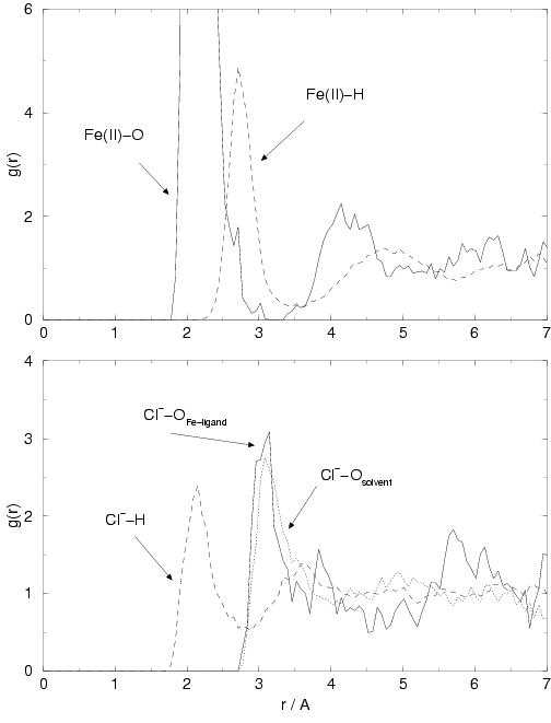
Figure 5.1 shows the radial distribution of water hydrogens and oxygens around the iron(II) cation (upper graph) and the two chloride anions (lower graph). The first peak in the Fe-O curve is centered at

Å and originates from the 6 water ligand oxygens in the coordination shell of Fe $^{\mathrm{II}}$ . None of these six ligands exchange with solvent molecules during our short simulation, which follows from the zero value of $g_{\mathrm{Fe-O}}$ at

Å. The peak position and the width at half height $\Delta_{\mathrm{FeO}}$ agree very well with the neutron diffraction data of a 1 molal iron chloride solution, shown in table 5.1. The little shoulders at the right hand side of the peak are probably due to the sharing of water molecules by iron and one of the chloride anions. Also Fe-O bond elongations due to Jahn-Teller distortions in the high-spin hexaaqua iron(II) complex could explain these little shoulders, but in that case simultaneous Fe-O bond elongations are expected for a pair of opposite water ligands. We did not find any evidence for such a correlation. The second peak arising from water molecules in the second iron shell is centered at 4.26 Å, which is slightly less than the 4.30-4.51 Å, obtained with x-ray diffraction [150]. Integration of the peak up to the shallow minimum at

Å gives 10.5 for the number of water molecules in the second solvation shell of iron. Note however, that the limited statistics of the short AIMD trajectory causes noise in this curve and in the location of the (relatively subtle) minimum which serves as the upper integration limit. Integration of a Gaussian fitted to this Fe $^{\mathrm{II}}$ -O peak gives a larger number of 11.67 water molecules. Integration of the first peak of the O $_{\mathrm{ligand}}$ -O $_{\mathrm{solvent}}$ radial distribution function (data not shown) results in 1.78 second shell water molecules per water ligand, i.e. 10.7 molecules in the second solvation shell of iron. The experimental number of 12 from X-ray diffraction of a frozen 55.5 H

O/FeCl

molar ratio solution is not very accurate, which follows from the deviation of least-squares fitted model of these authors to their measured data for distances larger than 4 Å.[173] The position and shape of the first Fe $^{\mathrm{II}}$ -H correlation peak arising from the 12 water ligand hydrogens agrees very well with neutron diffraction data (table 5.1). Although the minimum at

Å does not go to zero, no hydrolysis of the hexaaqua iron complex is observed during the simulation. The abundancy of hydrogen at a distance of

Å from the iron ion must therefore come from second shell water molecules.

**Table 5.1:** Structural properties of FeCl in water compared to experiment. and $\Delta$ are the position of the maximum and the full width at half maximum respectively of a Gaussian fitted to the radial distribution peak. is the coordination number derived from integration over the peak. $\Theta$ is the average tilt angle of the ligand water molecules, defined as the angle between the Fe-O axis and the bisector of the water molecule.

	$R_{\mathrm{FeO}}$ (Å)	$\Delta_{\mathrm{FeO}}$ (Å)	$n_{\mathrm{FeO}}$	$R_{\mathrm{FeH}}$ (Å)	$\Delta_{\mathrm{FeH}}$ (Å)	$n_{\mathrm{FeH}}$	$\Theta (^\circ)$


AIMD	2.134	0.263	6.0	2.762	0.371	12.1	38 $\pm$ 18

Neutron diff.	2.13	0.28	6.0	2.75	0.36	12.1	32 $\pm$ 15

1 molal iron(II) chloride in acidic heavy water solution.[148]

The lower graph shows the distribution of water molecules around the chloride anions. The first peaks of $g_{\mathrm{ClH}}$ and $g_{\mathrm{ClO}}$ originating from the first Cl

solvation shell are very similar to the ones from the radial distribution functions of HCl in water, published earlier [144]. The positions of the peak maxima $r_{\mathrm{ClH}}=2.1$ Å and $r_{\mathrm{ClO}}=3.1$ Å are identical. The main difference is that the present peaks are slightly less pronounced, i.e. they have a somewhat lower maximum and less deep minimum following the peak. Also the comparison with the neutron diffraction results on a 2 molal NiCl

solution is quite satisfactory ( $r_{\mathrm{ClH}}=2.28$ Å and $r_{\mathrm{ClO}}=3.1$ Å, respectively)[174], although the Cl-H peak is shifted a little to the right-hand-side and is also a little broader in the experiment, resulting in a coordination number of 6.4 for Cl

in NiCl

(aq). Integration over the $g_{\mathrm{Cl-H}}$ peak up to

Å result in a coordination number of

, slightly lower than the 5.2 found for the hydrochloric acid simulation.[144] This difference as well as the lack of the pronounced second shell structure in the present graphs, contrary to the HCl(aq) distribution, is the result of the higher concentration of structure making ions in the FeCl

(aq) simulation compared to the HCl(aq) one (the latter system contained 1 proton and 1 Cl

per 32 H

O). The presence of the hexaaqua iron moiety and the other Cl

anion in the neighborhood do not allow the first chloride to build the hydration structure beyond the first solvation shell in the same way as in a more dilute Cl

solution. On average, one (1.2) of the water molecules in the first solvation shell of Cl

, belongs to the hexaaqua iron complex. The iron(II) chloride distances vary between 3.5 and 6.5 Å, and the Cl-Cl distance varies between 5 and 8 Å. Note that the maximum distance two particles can separate in the periodic box is 8.63 Å.

One final structural property we mention is the orientation of the six ligand water molecules, defined as the average angle between the Fe-O axis and the bisector of the water molecule, $\Theta$ . This tilt angle fluctuates around 38 degrees with a standard deviation of 18 degrees, which is again close to the experimental number of 32 $^\circ \pm 15^\circ$ .

We conclude that AIMD with the BP functional and with the 30 Ry cutoff plane wave basis set is very well capable to describe the nearest solvent structure of high-spin iron(II).